I’ve had the pleasant experience of working in a fluid mechanics laboratory for the past two-and-a-half months, and this lab was primarily focused on schooling behavior of fish due to hydrodynamic interactions. I had originally intended to do something a bit more fundamental in fluid mechanics so that I could learn some fluid physics while working, but interestingly, their concern on fish dynamics is actually far more of a particle simulation problem.

The issue they tasked me with solving is fairly simple and purely computational: real fish schools are far larger than they could simulate using straightforward, brute-force calculations. They were interested in modelling only passive hydrodynamic interactions between fish (so ignoring behavioral factors or active effects like vortical wake), but any simulation system consisting of \(N\) point-masses (or similar) where each point-mass effects each other point mass requires the calculation of \(N^2\) interactions per time-step. This is, by definition, the \(N\)-body problem as seen in countless situations in computational physics, and as anybody who has ever dealt with this problem will tell you, it is the greatest bottleneck performing any computational research in particle-based systems. In particular, in this lab, they couldn’t get much farther than tens of thousands of swimmers: numbers around fifty thousand fish were considered quite high for simulation, and most of the research in the lab focused on less then fifty (often only two). This is a massive problem for research into this field, however, as real fish schools have been found to contain hundreds of millions of swimmers, thus leaving a massive gap in research as group sizes in the tens of thousands are puny compared to the hundreds of millions.

Therefore, I was tasked with creating a simulation program efficient enough to handle hundreds of millions of swimmers by using standard computational particle dynamics techniques, such as implementing the Barnes-Hut algorithm, the Fast Multipole Method, and using parallel and/or distributed computing. This led to the creation of FINDS, a C library for performing fast simulation of large schools.

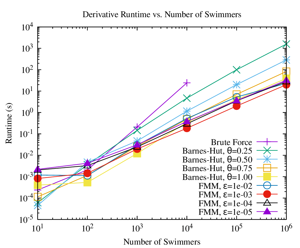
This library brings the computation time for the derivative of a system down from a time complexity of \(O(N^2)\) to \(O(N \log N)\) and \(O(N)\) using the Barnes-Hut approximation and the Fast Multipole Method respectively, and this translates into a difference in computation time from hours or days per computation to seconds at scales at or above \(10^5\) fish (see the figure below).

FINDS by example

The way that FINDS works is incredibly simple, and I’ll use the example imploding_sphere.c.

First, we can load in all of FINDS with the header <finds/finds.h>, but each individual module can be loaded in manually. The beginning system configuration is manually defined by the user, and this can be done by setting the distribution, orientation, and constant options to define standard schools or by manually setting the parameters for each fish in the system.

In this case, we want to produce a sphere that implodes upon itself, i.e., what we can see in the figure below.

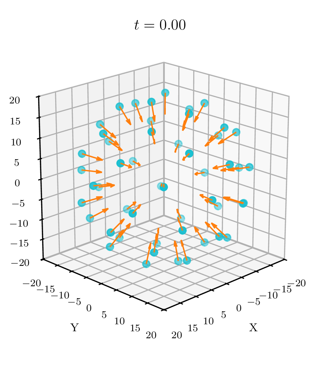
To do this, we first need to set a spherical distribution (a fibonacci sphere) with the following code:

distribution_options_t dist_opts = {0};
dist_opts.type = DISTRIBUTION_SPHERE;
dist_opts.radius = RADII;
dist_opts.spacing = SPACING;

Then, we set the orientation of the fish to all face the origin:

orientation_options_t ori_opts = {0};
ori_opts.type = ORIENTATION_RADIAL_INWARD;

And then, lastly, we set the fish to all be uniform in length and volumetric flow rate:

constant_options_t const_opts = {0};
const_opts.random_length_selection = false;
const_opts.uniform_length = 1.0;
const_opts.random_volumetric_flow_selection = false;
const_opts.uniform_sigma = 4 * M_PI;

Then, we build the overall initial system:

fish_system_t *system = fish_system_generate(
    dist_opts, ori_opts, const_opts, true);
if (!system)
    return EXIT_FAILURE;

Now, all that is necessary is determining how we compute the derivative of each state and how we will integrate this derivative to compute each next state. Per the derivative scaling figure above, it would be ideal to compute the derivative using the Barnes-Hut algorithm with a high approximation ratio, \(\theta=1.0\), as the initial overhead is considerably low.

derivative_computation_opts_t dc_opts = {0};
dc_opts.method = BARNES_HUT;
dc_opts.approximation_threshold = 1.0;
dc_opts.regularize = true;
dc_opts.regularization_epsilon = 1E-6;

Then, for the integrator, we can pick a basic non-adaptive integrator as this is a fairly stable system (up until the point of implosion, at which it becomes extremely unstable, making regularization would be necessary):

integration_opts_t int_opts = {0};
int_opts.method = RUNGE_KUTTA_4;
int_opts.eval_time_step = 1.0;
int_opts.end_time = 100;
int_opts.print_time_progression = true;

With all of that setup, we can perform the simulation, and this returns the filename of the produced trajectory data in HDF5 format:

char output_folder_name[BUFFER_SIZE];
char output_filename[DOUBLE_BUFFER_SIZE];

errcode = perform_simulation(
    system, dc_opts, int_opts,
    output_filename, output_folder_name,
    BUFFER_SIZE, DOUBLE_BUFFER_SIZE, false);
if (errcode != ERR_OK) {
    puts("Error occurred! Dataset is likely corrupted.");
    goto jmp_system;
}

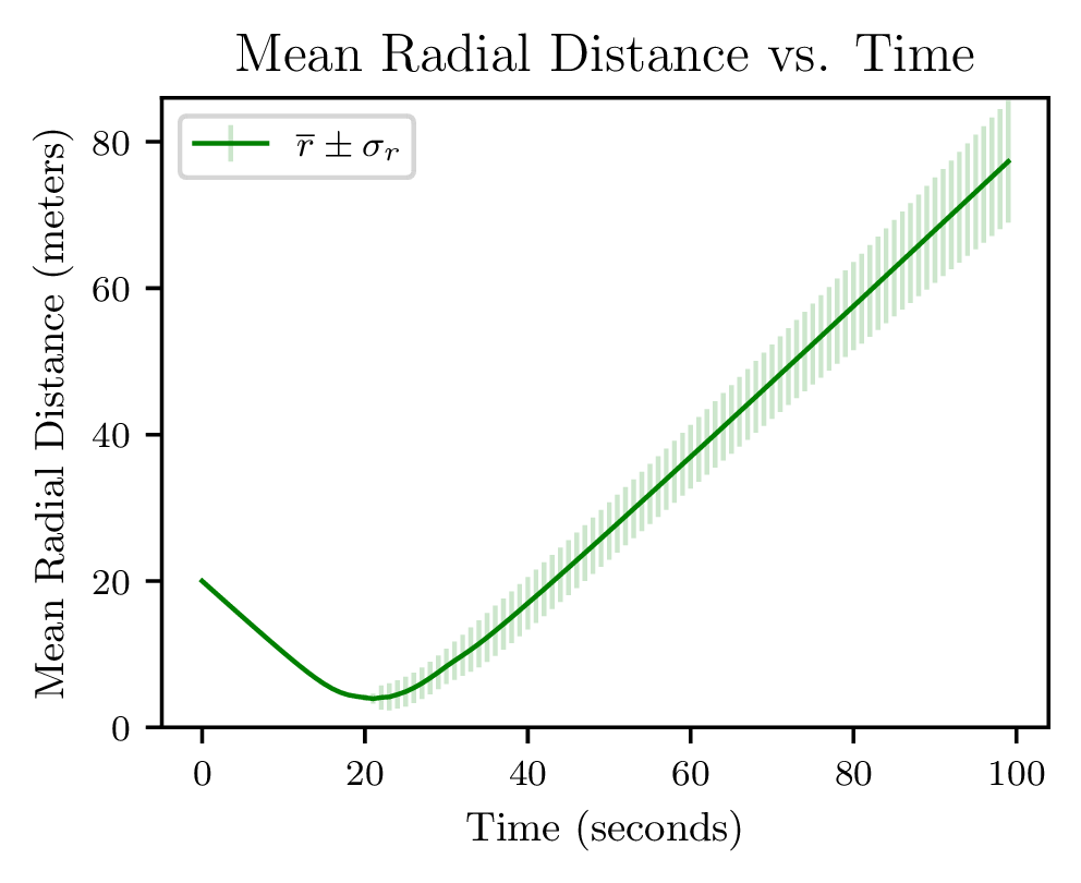
And after performing a simulation, we can run the post-processing modules on the produced dataset with make analyze file={ouptut_filename}, and this produces analysis figures like a plot of the mean radial distance, animations, etc.

Locating FINDS and the Manuscript Pre-print

For more in-depth information, the FINDS documentation can be found online (Online Link) and the pre-print manuscript describing FINDS can also be found here (PDF).