Paper Explanation

I have had a lot of fun with The Laws of Thermodynamics, a compilation of contemporary articles within the field. This wasn’t really the kind of book you’re intended to read front-to-back like a novel, but skim for articles that you find interesting and then really devour them. Of these, one article really caught my eye: a proposition for a quantum-mechanical carnot engine [1].

Most of the calculations went way over my head, but I could follow little bits and pieces of the logic. To help with this, I’ve made a bit of some python code so that this can actually be run, and placed it under each write-up section or calculation, and it includes the following imports:

import numpy as np
from scipy import constants
from matplotlib import pyplot as plt

To understand this post, I recommend reading it somewhat like you would a Jupyter notebook.

Now, firstly, basic quantum mechanics follows that any quantum object or system is the sum of eigenstates (the writers of this paper based their logic upon there being infinitely many eigenstates, but for our calculations, we’ll be using a finite number). Each eigenstate can be denoted an indexing number \(n\), that being, its principal quantum number (if this were modelling an electron, for example, this would be its energy level). The principal quantum number of an eigenstate relates to the energy at that state using the energy spectra equation

def calculate_energy(mass, level, width):
    return (np.pi * constants.hbar * level) ** 2 / (2 * mass * width)

where \(V\) is the volume of the potential well that the wavefunction inhabits (which, in only one dimension, is synonymous with the width or length of the well, which we will denote \(w=V\)) and \(m\) is the mass of the particle/quantum object.

From there, we can calculate the probability distribution of eigenstates with

def prob_dist(mass, temp, width, max_level):
    partition_function = [pf(mass, temp, width, n) for n in range(1, max_level+1)]
    pf_sum = sum(partition_function)
    return [pf_eigen/pf_sum for pf_eigen in partition_function]

based on the energy-partition function

def pf(mass, temp, width, level):
    return np.exp(-calc_energy(mass, level, width) / (constants.Boltzmann * temp))

and in-turn, this allows us to calculate the von Neumann entropy as a function of the well-width \(w\) and the engine temperature \(T\) as

def calculate_entropy(mass, temp, width, max_level):
    return -sum(prob * np.log(prob) for prob in prob_dist(mass, temp, width, max_level))

Then, therefore, with these equations in mind, we can create the Carnot cycle quantum-mechanically using a time-dependent cyclic hamiltonian performing the following four thermodynamical transformations

1. Isoenergetic Expansion (notice its similarity to the classical isothermal transformation),
2. Adiabatic Expansion,
3. Isoenergetic Compression, and
4. Adiabatic Compression,

and cycles each of the variables in the system between various states:

1. The width of the system cycles from \(w_1\), the initial width, to \(w_2\), the width of after the isoenergetic expansion, and \(w_3 = w_2 \sqrt{T_H/T_C}\), the width after the adiabatic expansion, and \(w_4=w_1 \sqrt{\frac{T_H}{T_C}}\), the width after the isoenergetic compression (and \(w_1\) is simultaneously the width after the final adiabatic compression).
2. The temperature of the system transfers between \(T_C\), the energy of the cold bath, and \(T_H\), the energy of the hot bath (as it would in a classical Carnot cycle).

M = constants.physical_constants['proton mass'][0]
NMAX = 20
W1 = 1e-10
W2 = 2e-10
TH = 300
TC = 150 

Therefore, as each quantum-thermodynamical state can be represented as a function of just the width and temperature of the engine, we can define the following states associated with the point before each transformation:

1. Initial state: \((w_1, T_H)\)

S1 = calculate_entropy(M, TH, W1, NMAX)

1. After the isoenergetic expansion: \((w_2, T_C)\)

S2 = calculate_entropy(M, TC, W2, NMAX)

1. After the adiabatic compression: \(\left(w_2 \sqrt{\frac{T_H}{T_C}}, T_C\right)\)

S3 = calculate_entropy(M, TC, W2 * np.sqrt(TH/TC), NMAX)

1. After the isoenergetic compression: \(\left(w_1 \sqrt{\frac{T_H}{T_C}}, T_H\right),\)

S4 = calculate_entropy(M, TC, W1 * np.sqrt(TH/TC), NMAX)

and these states can therefore be plotted on a width vs entropy graph to show the cycle, as the researchers did.

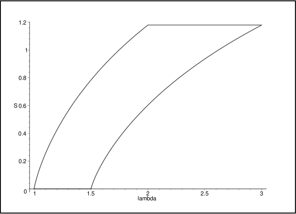
plt.plot([W1, W2, W2 * np.sqrt(TH/TC), W1 * np.sqrt(TH/TC)], [S1, S2, S3, S4])
plt.show()

My thoughts

The reason why I was able to follow any of that is that I went and made a bit of some python code to replicate it. I wrote up a jupyter notebook to try and follow this, as you can see from the code above, but I’m still woefully confused on what was going on. A lot of the math went way over my head, and this was a severe oversimplification of their work. Really, this is just what I could make from it. Anyway, I thought it was cool, and I had fun doing this.

What I think I really learned from this, surprisingly, is the important of quantum units for quantum mechanical calculations. The reason why NMAX is so small (only 20 eigenstates considered) in the code is because the floating-point calculations are just too difficult. If I could have performed the calculations in quantum units, I could have raised NMAX considerably higher as all of the floating-point calculations would be raised tens of magnitudes higher, making all of the calculations much more precise (and somewhat realistic). I learned, essentially, that quantum units aren’t just something scientists do to make their lives easier, they are a necessity to perform any quantum calculations whatsoever.

There’s probably a lot of problems with what I wrote, and if you find something you want me to change (without being nitpicky), feel free to email me.

[1] “Entropy and Temperature of a Quantum Mechanical Carnot Engine” by Bender et al. arXiv