Flashback to last year. I took a physics laboratory course that would routinely hand me new functions for fitting nearly every week, and with each new week, I continued to build a growing, monstrous Python file containing each of these analysis routines. I called this file common.py, and as the file grew, it became incredibly cumbersome and annoying to try and manage everything, so I had to start going back into the file and generalizing everything with classes and generics and such. When this first lab class ended, I thought that I was done with having to bother with these for good, but following the end of the class, my immediate next lab course required the same work, so I started again with a fresh common.py that seemed to grow even larger and faster than the previous one did. At that point, I got fed up, and just did a little Sphinx magic to finally document and formalize this franken-file of jumbled up functions into a proper library for data analysis called Experimentalis.

The way that the library works is very, very simple. It’s based on two key data types: datasets and models, and the whole point is building a big repository of various models to fit to various models to approximate parameters.

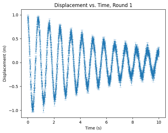
Some examples are included with the project’s GitHub repository, but I’ll illustrate two of them here as well. Imagine I have some noisy dataset that I believe matches some known form (which can be an analytical function or some differential equation) such as the case of a damped harmonic oscillator:

Now, assuming I have some arrays t, y, dx, and dy containing the time values, the amplitude-values, and the uncertainty in the time-values for each measurement, I can build a Dataset object to store this full dataset:

dataset = Dataset(
    x=t,
    y=y,
    dx=dx,
    dy=dy
)

Then, I can make some guesses on this dataset based on first principles or background knowledge or etc. I already know that this dataset should be the result of a damped harmonic oscillator, so I’ll be fitting a model of the form

where \(A\) is the amplitude, \(\tau\) is the time/damping constant, \(f\) is the frequency of oscillation, and \(\phi\) is the phase. I could do some simple mathematical analysis or simply guess to develop some simple guesses for where each parameter realistically should be, and in this case, our guesses can safely end up being \(A = 0.8, \tau = 0.1, f = 1,\) and \(\phi = 0\). From that, we can make our model:

model = DampedHarmonicModel(
    amplitude = 0.8,
    time_constant = 0.1,
    frequency = 1.0,
    phase = 0
)

and now, all we need to do is just fit the model to the data, and see what happens:

result = autofit(dataset, model, graphing_options=g_opts)
print_results(model, result, units=['m', 'Ns/m', 'Hz', 'rad'])

And the output of this yields \(A = 1.0, \tau = 0.15, f = 1.2,\) and \(\phi = 0.3\) for \(\chi^2 = 1.0\), and we get the following plot:

display(result.autofit_graph)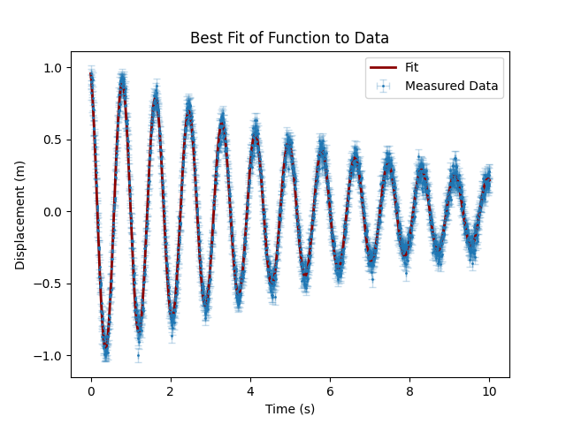

showing that this fit really did work as-intended, and the parameters we obtained are reasonable.

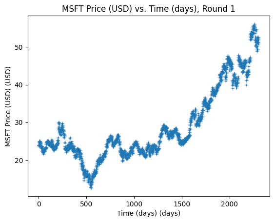
Now, what is incredibly important to keep in mind here is that fundamentally, this data is just a one-dimensional series. This means that we can very easily make new models for fitting all kinds of one-dimensional series, such as time-series, and a very classic example of this is in stock market prediction. A fairly trivial model for stock markets, in particular, is Geometric Brownian Motion from Stochastic Calculus, and similarly to before, we can also use this library to fit a GBM model to real stock data. Once again, presume we have some stock data on Microsoft as loaded in this form:

prices = df[stock].values
dates = np.arange(len(prices))

returns = np.diff(prices) / prices[:-1]
noise_std = np.std(returns)

dataset = Dataset(
    x=dates,
    y=prices,
    dx=np.full_like(dates,  2/24),
    dy=np.full_like(prices, noise_std)  # small assumed measurement uncertainty
)

which looks like the following:

We can then build a simple GBM based on assuming 2% volatility (\(\sigma=0.02\)) and 0.11% drift (\(\mu=0.0011\)):

model = GBM(
    initial_value = prices[0],
    drift = 1.1e-3,
    drift_bounds = (0,0.1),
    volatility = 2e-2,
    volatility_bounds = (0,1)
)

Then, we can just let it run buck-wild on this data:

result = autofit(dataset, model, graphing_options=g_opts)
print_results(model, result)

and this actually won’t change the model parameters we gave it due to the fact that its a stochastic model (so there are local minima essentially everywhere, making curve_fit useless), but it can give some really interesting potential fits:

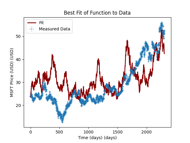
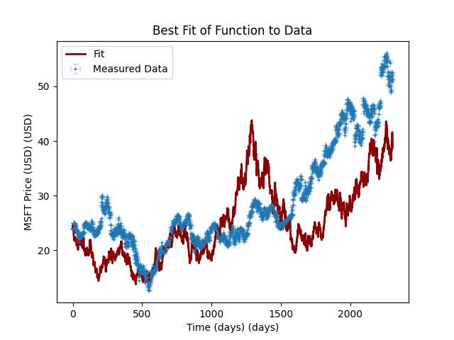
However, each at a substantial price: \(\chi^2 > 5 \times 10^7\). Again, though, this is to be expected, as this is a very naive model, so it is entirely to-be-expected that it wouldn’t work.